From Perceptrons to ChatGPT: Neural Networks Evolve

Neural networks have more than 80 years of history. Today’s systems are not the product of one invention. They combine a formal neuron from 1943, the perceptron, multilayer representation learning, convolution, GPUs, large datasets, residual connections and attention. Neural networks were repeatedly declared both the future of AI and a dead end. Both judgements arrived too early.

This article explains the technical sequence without hiding behind equations. It also shows why the history matters in production: architecture does not repair poor data, a benchmark is not a security guarantee and a deeper network does not necessarily “understand” more.

Neural-network timeline

Year	Stage	Contribution
1943	McCulloch–Pitts	A logical threshold-neuron model
1949	Hebb	Connections strengthen through correlated activity
1957–1958	Rosenblatt’s perceptron	A classifier learns weights from examples
1969	Minsky and Papert’s “Perceptrons”	Formal limits of single-layer networks
1986	Backpropagation	Practical learning of useful hidden representations
1989–1998	LeNet and CNNs	Shared weights and local filters for images
2012	AlexNet	GPUs, data and a deep CNN transform ImageNet
2015	ResNet	Residual connections enable much deeper training
2017	Transformer	Self-attention scales sequence modelling

1943: a neuron as a logical function

Warren McCulloch and Walter Pitts modelled a neuron as a binary element: input signals are combined and the output activates when a threshold condition is met. Networks of these units could implement logical operations. This was an abstraction rather than a faithful simulation of biology, but it established that network behaviour could be analysed formally.

In 1949 Donald Hebb described learning in terms associated with strengthening connections between neurons that are repeatedly active together. Modern training algorithms are not simple implementations of Hebbian biology, but the notion that knowledge can be encoded in connection strength became central to connectionism.

The distinction still matters. A contemporary artificial “neuron” is a numerical function applying a weighted sum and non-linearity. The biological label is a useful metaphor, but it can also encourage unwarranted claims about minds and consciousness.

The perceptron learns its own weights

Frank Rosenblatt developed the perceptron in the late 1950s. It takes features, computes a weighted sum and selects one of two classes. When a prediction is wrong, its learning rule moves weights towards the correct decision. For linearly separable data, the learning procedure converges.

Media enthusiasm exceeded the method’s scope. A single-layer perceptron cannot represent problems that cannot be split with one hyperplane; XOR is the standard example. Marvin Minsky and Seymour Papert formally described important limitations in their 1969 book. Popular retellings say the book “killed” neural networks, but that is too simple. It analysed a specific class of model and acknowledged that multilayer networks could overcome some limits; the practical training method and computing resources were not yet in place.

The first modern lesson is precision. “AI cannot do X” and “AI has solved X” are almost meaningless without an architecture, data distribution and acceptance criterion.

Hidden layers and assigning responsibility for error

A multilayer network can represent complex decision boundaries. The challenge is determining which hidden connection contributed to an output error. Backpropagation uses the chain rule. A forward pass produces an output, a loss function measures error, and gradients of that loss are propagated from the output back through every parameter. An optimiser then adjusts parameters to reduce the loss.

In 1986 David Rumelhart, Geoffrey Hinton and Ronald Williams published an influential demonstration of this procedure learning useful hidden features. The idea had earlier roots, so it is more accurate to describe the paper as a landmark in popularising and demonstrating backpropagation than as a single moment of invention.

Backpropagation does not guarantee a globally optimal model. Training depends on initialisation, gradient scale, activation functions, data and hyperparameters. Vanishing and exploding gradients hindered deeper networks for years. Better activations, initialisation, normalisation and architecture gradually made optimisation more reliable.

Convolution embeds useful assumptions about images

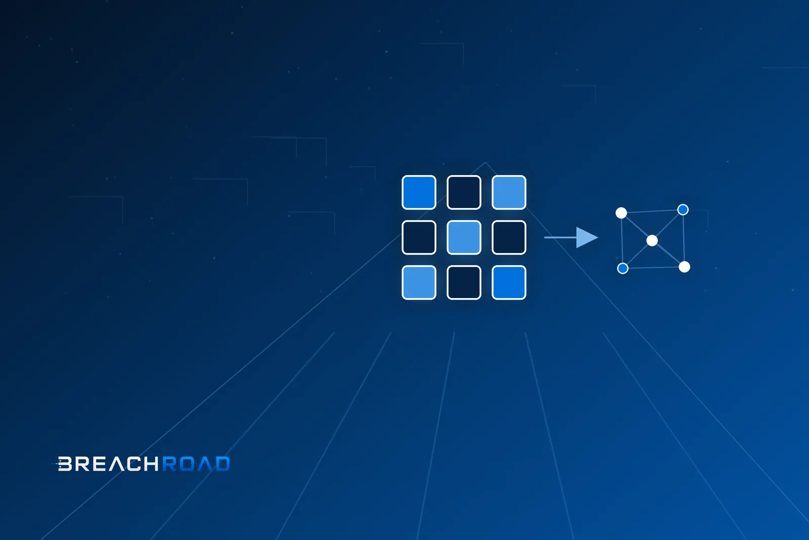
Connecting every pixel to every unit produces an enormous parameter count. Convolutional networks use two image properties: patterns are local and the same pattern may appear in different positions. A small filter moves across an image and reuses the same weights. This weight sharing reduces parameters and injects an appropriate structural bias.

Yann LeCun and colleagues demonstrated gradient-based document recognition with systems such as LeNet-5, combining convolution, downsampling and classification. It was evidence that neural networks could solve a narrow production task long before the 2012 boom.

Why AlexNet arrived in 2012

AlexNet was not the first CNN. Its breakthrough came from combining enough labelled data, GPU computation and practical design choices. The authors trained on roughly 1.2 million ImageNet images across 1,000 classes. The network used around 60 million parameters. GPUs accelerated convolution, ReLU aided optimisation, augmentation reduced overfitting and dropout randomly removed activations during training.

Its ILSVRC 2012 top-5 error was markedly stronger than competing systems. The margin convinced researchers and industry that learned representations could outperform pipelines based on hand-engineered features. Deep learning then expanded rapidly across vision, speech and language.

Success also exposed the cost. Large networks need data, energy, time and specialist infrastructure. If labels are wrong or samples do not represent deployment, scale amplifies confidence rather than correcting assumptions.

ResNet makes much deeper networks trainable

Adding layers did not always improve results. Even without overfitting, very deep networks could become harder to optimise. ResNet introduced residual blocks. Rather than learn an entire transformation directly, a block learns a residual update while an identity shortcut carries the input forward. This simple route helps information and gradients move through the model.

Residual connections enabled practical training of networks tens or hundreds of layers deep and influenced architectures beyond CNNs. The engineering lesson is broader: progress often comes not from adding more of the same component, but from redesigning the path through which information flows.

Transformers model relationships in a sequence

Recurrent networks process sequences step by step, limiting parallelism and making distant relationships difficult. The 2017 Transformer used self-attention. Each token produces query, key and value representations. Compatibility between queries and keys determines weights used to combine values; multiple attention heads can learn different relationships.

Because attention alone does not encode order, positional information is added. Layers combine attention, feed-forward networks, normalisation and residual paths. The architecture uses accelerators efficiently and became the base of modern language models. The wider arc is covered in our complete history of AI.

Transformers scale sequence prediction, not truth. A model can produce fluent falsehoods, remain vulnerable to prompt injection, and execute unsafe instructions when an application grants overly broad tools.

From task-specific classifiers to foundation models

Traditional models learned one labelled task. A foundation model learns broad representations from a large corpus and is adapted through examples, instructions, fine-tuning or retrieval. One base can power many products, but shared capability also creates shared risk.

Application quality now depends on the model, system prompt, retrieval pipeline, permissions, filters, memory and integration code. An LLM security assessment therefore cannot be a list of jailbreak prompts. It must follow data and actions to their real-world effect.

Security lessons from this history

A representation is not an explanation. Accuracy does not reveal why a model chose an answer.
Training data is part of the attack surface. Poisoning, weak labels and leakage can alter behaviour.
A benchmark is a sample, not a warranty. Teams need domain tests, edge cases and regression suites.
Models must not enforce their own permission boundaries. Deterministic access control belongs outside the model.
Observability is essential. Without inputs, retrieved context, tool calls and outputs, an incident cannot be reconstructed.

Those principles inform secure enterprise LLM deployment and AI red teaming.

Frequently asked questions

Does a neural network work like a human brain?

Only in a loose inspirational sense. An artificial neuron is a simple mathematical function. Its training, scale and organisation differ greatly from biology. The metaphor is educational, not evidence of consciousness.

Who invented backpropagation?

It has a multi-stage history with important earlier work. Rumelhart, Hinton and Williams’ 1986 paper became a particularly influential demonstration of learning representations by propagating error. Crediting the entire method to one person would be misleading.

Why did neural networks not succeed in the 1960s?

Digital data, cheap computing, mature optimisation techniques and architectures that support deep training were not available together. Single-layer perceptrons also had real representational limits.

Is a larger model always better?

No. Scale can improve many capabilities while increasing cost, latency and control difficulty. Data, objective, evaluation and system design remain decisive. A smaller model may be safer, faster and cheaper for a narrow function.

Sources

Building a neural, retrieval or agentic system? Explore our AI red-team service, which tests the model together with its data, tools and access controls.